Calculation of the Derivatives
Test Cases for the Procedures Derivs and DerivsThruCPT
1) The first test of the derivative calculation algorithms is the case given in The NURBS Book's Figure 3.15.
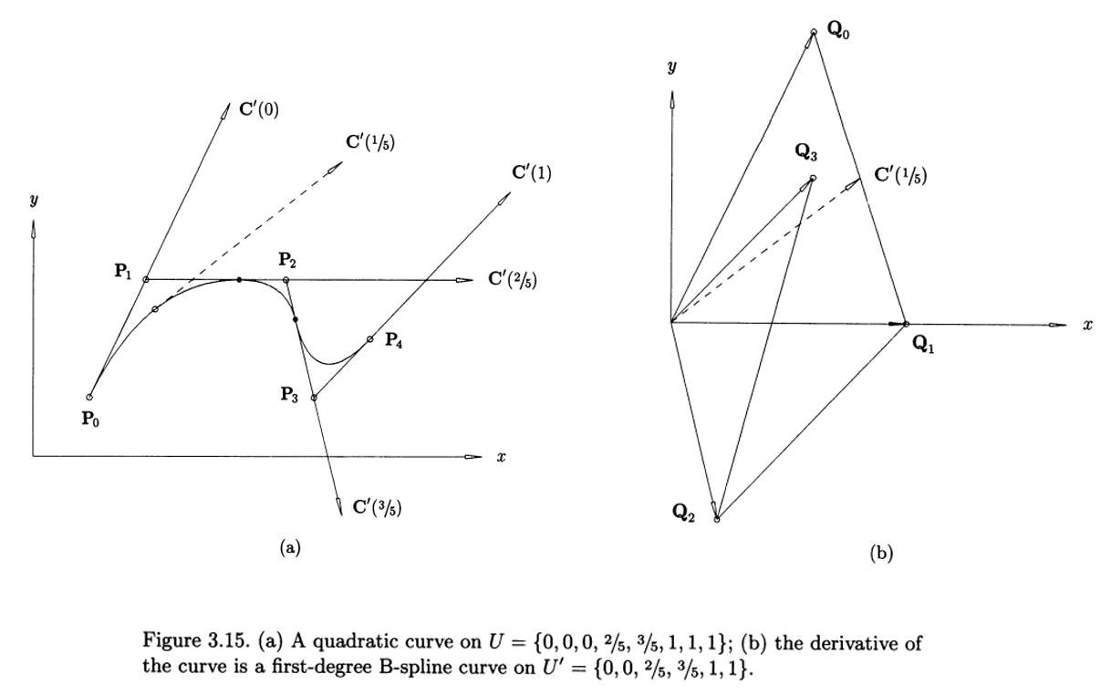
The following test program reproduces this case by using several ways.
program test_curve_derivative_calculation

use splines
use points

implicit none

integer, parameter :: wp  = selected_real_kind(15,307)
real(wp)  :: U(8)
type(curve) :: c,dc
type(cpt) :: D(0:1),D2(0:1)
type(cpt) :: a(5)
type(cpt) :: BK(0:1,0:4)

!control points of the curve
a(:)%x = [1., 2., 4., 4.5, 5.5]; a(:)%y = [1., 3., 3., 1., 2.]

!the knot vector U={0,0,0,0.4,0.6,1,1,1}
U=[0.0_wp, 0.0_wp, 0.0_wp, 0.40_wp, 0.60_wp, 1.0_wp, 1.0_wp, 1.0_wp]

!construct quadratic curve on U={0,0,0,0.4,0.6,1,1,1}
c = spl(dim=2, pd=1, p=[2], kXi=U, cp=a)

!calculate the control points of the curve derivative, BK(1,0:4)
call c%DerivCpts(d=1, BK=BK)

!construct linear curve on U'={0,0,0.4,0.6,1,1}
!by using the control points of the first derivative curve
dc = spl(  dim=2, pd=1, p=[1], &
            kXi=U(2:ubound(U,1)-1), &
            cp=BK(1,0:3))

!calculate C^(k) (u=0), k=0,1
call c%Derivs       (u=0.0_wp, d=1, CK=D)
call c%DerivsThruCPT(u=0.0_wp, d=1, CK=D2)

!plot the curve
call c%plot(    plotCP=.true., labelCP=.true.,derivs=[0], &
                    terminal='png',                 &
                    fname="test_F3.15a",&
                    title="A quadratic curve")

!plot the shape functions of the curve with a hundred calculation points
call c%N(1)%plot(   terminal='png',                 &
                        fname="test_F3.15c",&
                        title="Basis functions of the quadratic curve")

!plot the derivative curve
call dc%plot(   plotCP=.true., labelCP=.true., &
                    terminal='png',                 &
                    fname="test_F3.15b",&
                    title="The derivative of the quadratic curve")

!plot the first derivative of the curve
!it is identical with the previous plot
call c%plot(plotCP=.true., labelCP=.true., derivs=[1])

!plot the shape functions of the derivative curve
call dc%N(1)%plot(  terminal='png',                 &
                        fname="test_F3.15d",&
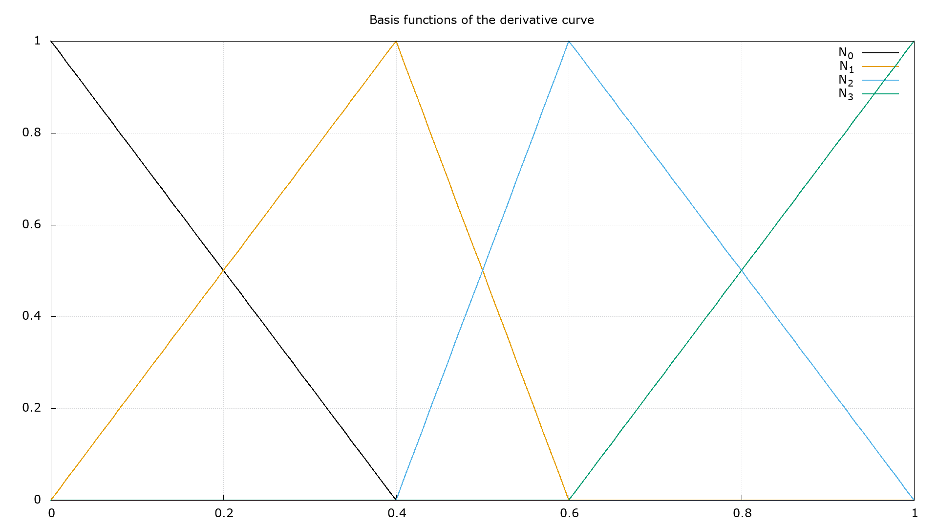
                        title="Basis functions of the derivative curve")

!curve point through `curve%Derivs` => C^(0) (u=0)
write(*,'(4(1x,f12.5))') D(0)%x, D(0)%y, D(0)%z
!=> 1.00000 1.00000 0.00000

!1st derivative through `curve%Derivs` => C^(1) (u=0)
write(*,'(4(1x,f12.5))') D(1)%x, D(1)%y, D(1)%z
!=> 5.00000 10.00000    0.00000

!1st derivative through the derivative curve (dcurve)
!constructed by using the `curve%DerivCpts` => C^(1) (u=0)
write(*,'(4(1x,f12.5))') dc%B(0)%x, dc%B(0)%y, dc%B(0)%z
!=> 5.00000 10.00000    0.00000

!1st derivative through `curve%DerivsThruCPT`  => C^(1) (u=0)
write(*,'(4(1x,f12.5))') D2(1)%x, D2(1)%y, D2(1)%z
!=> 5.00000 10.00000    0.00000

pause

end program test_curve_derivative_calculation
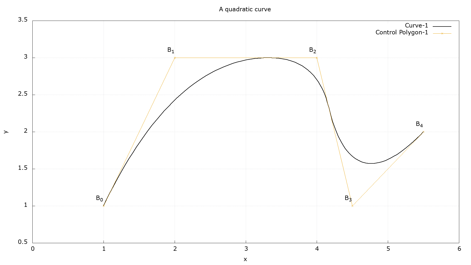
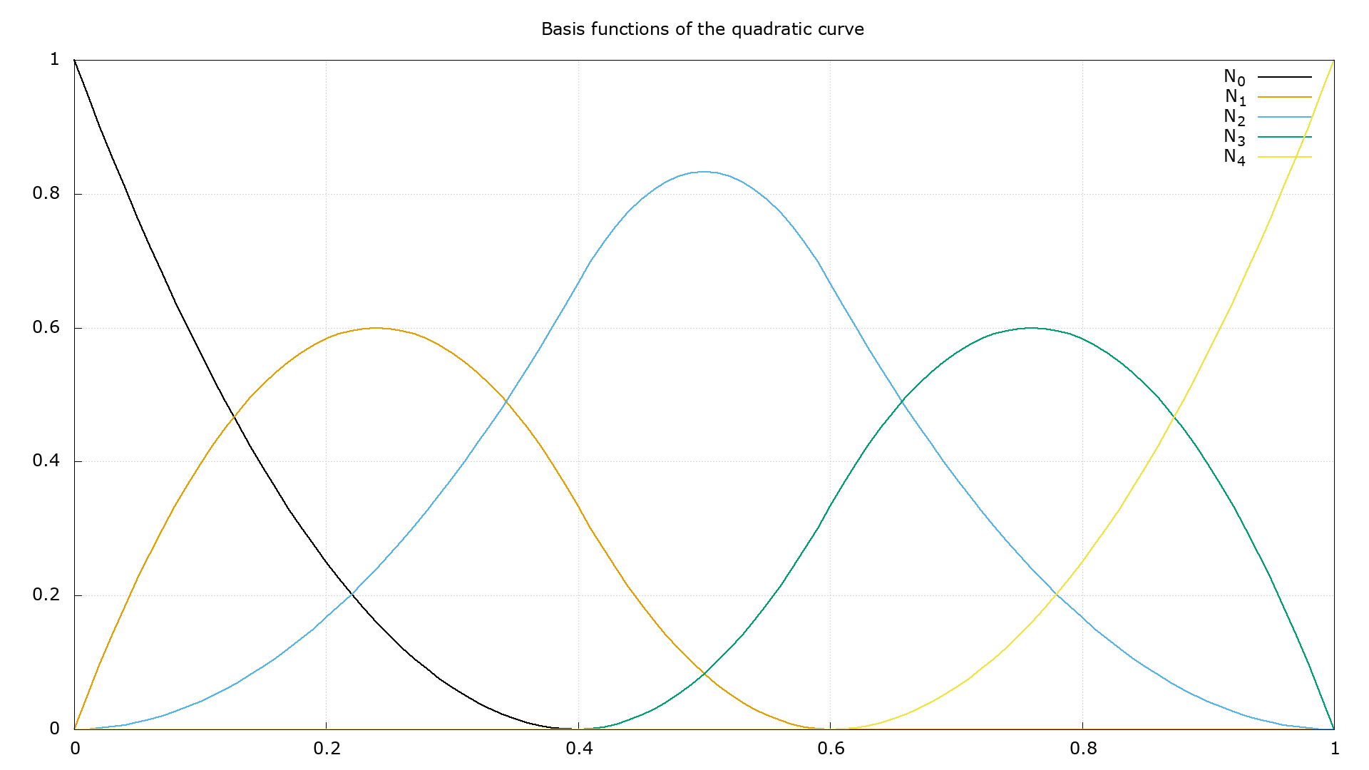
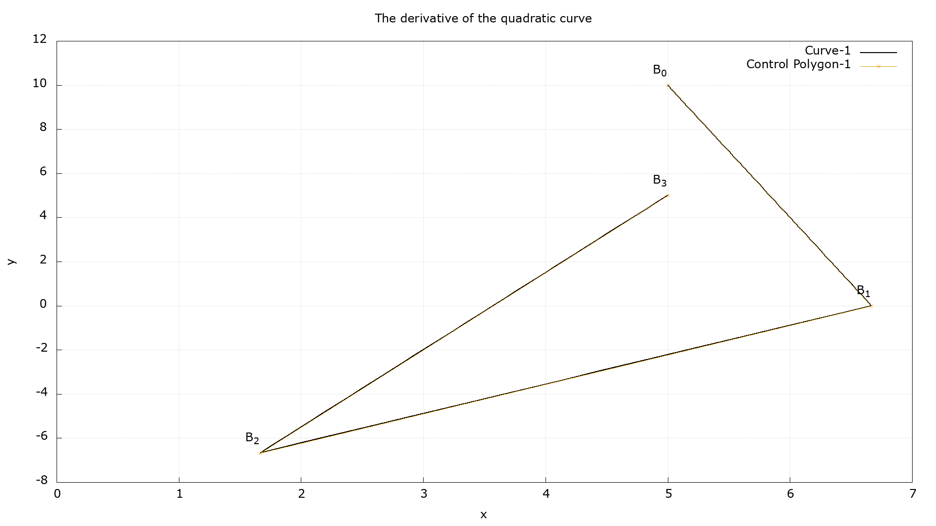
The output plots of the test_curve_derivative_calculation program are as follow,
The following test program ...
program test_surface_derivative_calculation
type(spl) :: surface
type(cpt) :: point(0:2,0:2)
real(wp)  :: a(9,2)

a(:,1) = [ 0., 0., 1. , -1., -1., 1., -2., -2., 1.] !u-coordinates
a(:,2) = [ 0., 1., 1.5,  0.,  2., 4.,  0.,  2., 5.] !v-coordinates

surface = spl(dim=2,pd=2,p=2,kXi=[0., 0., 0., 1., 1., 1.], &
     kEta=[0., 0., 0., 1., 1., 1.],cp=a,rational=.false.)

call surface%SurfaceDerivsAlg1(u=0.5,v=0.25,d=2,point)

write(*,'(4(1x,f12.5))') point(2,0)%x, point(2,0)%y, point(2,0)%z ! d^2[S(0.5,0.25)]/dx^2
write(*,'(4(1x,f12.5))') point(1,1)%x, point(1,1)%y, point(1,1)%z  ! d^2[S(0.5,0.25)]/dxdy
write(*,'(4(1x,f12.5))') point(0,2)%x, point(0,2)%y, point(0,2)%z  ! d^2[S(0.5,0.25)]/dy^2

end program test_surface_derivative_calculation